
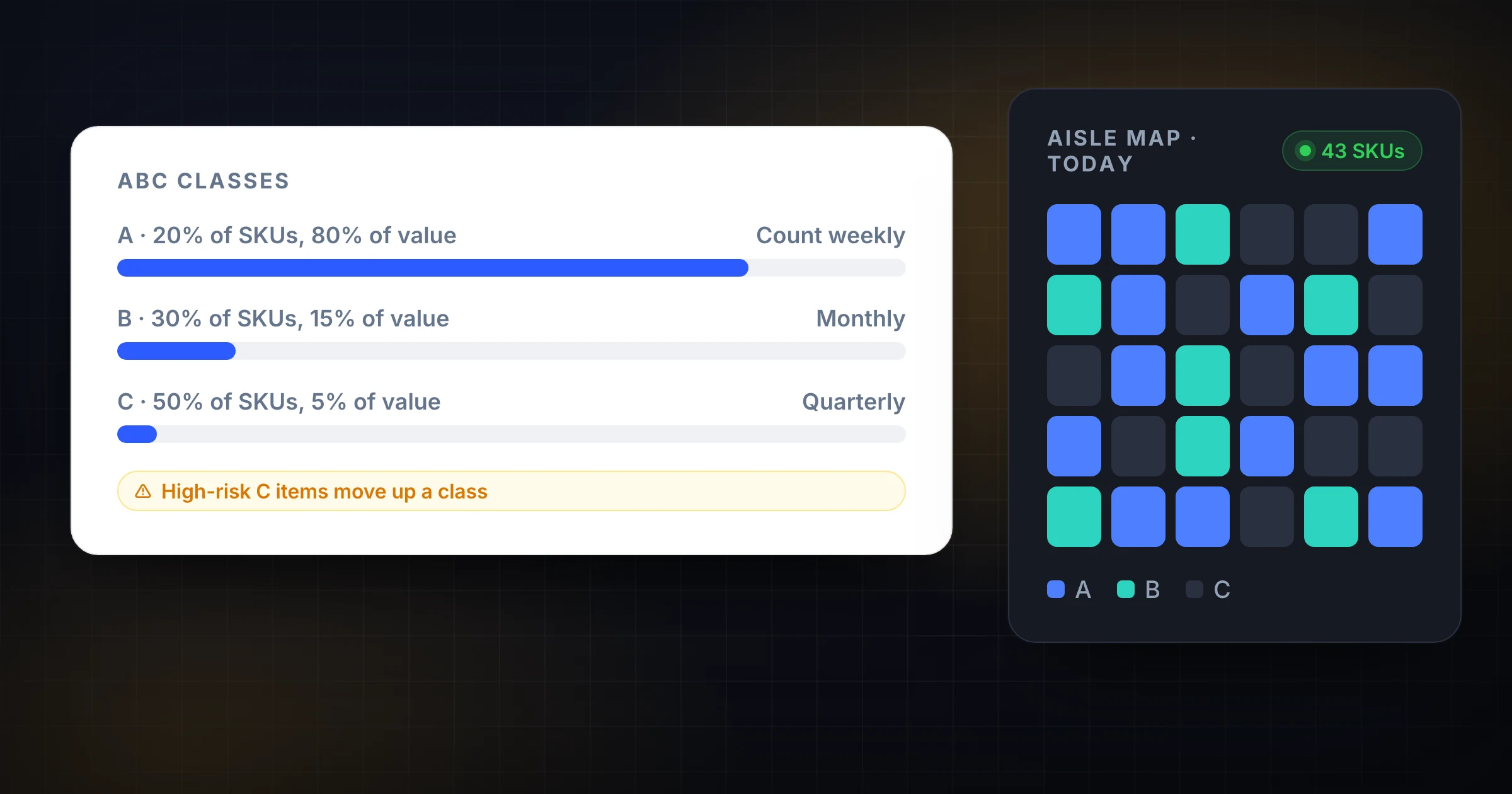
ABC analysis in cycle counting is how you stop treating every SKU like it deserves the same attention.
In most warehouses, a small group of items drives most of the value, movement, or customer pain. Those items should be counted more often. Slow-moving, low-value items still matter, but they should not consume the same daily count capacity as the parts that delay orders, tie up cash, or create expensive write-offs.
This guide shows you how to use ABC analysis for cycle counting in inventory management: how to classify SKUs, set count frequency, build the daily schedule, and avoid the mistakes that make ABC programs look precise but fail on the floor. If you are still building the basics, start with our guide to what cycle counting means. If you already count daily, use this as the next layer.
What ABC analysis means in inventory management
ABC analysis is an inventory classification method. It sorts SKUs into three groups based on importance:
- A items: the highest-value or highest-impact SKUs. They get the tightest control and the most frequent counts.
- B items: meaningful SKUs that matter, but do not deserve daily attention.
- C items: the long tail. They are still counted, but less often and with simpler controls.
The method is usually based on the Pareto principle. In plain terms, a minority of items often accounts for the majority of value or activity. Inventory consultant Dave Piasecki describes ABC classification as a practical way to focus attention when you have a lot of SKUs and limited management time in his guide to ABC classifications.
The key phrase is "focus attention." ABC analysis is not just a finance report. For cycle counting, it should decide which items get counted weekly, monthly, quarterly, or annually.
Why ABC analysis belongs inside cycle counting
Cycle counting gives you a daily rhythm. ABC analysis decides where that rhythm should be spent.
Without ABC classification, many teams create a simple rotation: count aisle 1 this week, aisle 2 next week, and so on until the building is covered. That is better than an annual physical count, but it misses the economic reality of the warehouse.
A $900 component that ships every day and blocks customer orders if it is wrong should not wait six months for its turn. A $2 spare label roll that moves twice a year does not need monthly attention.
ABC cycle counting fixes that mismatch. It lets you:
- Count expensive and high-velocity SKUs before small errors become big adjustments.
- Keep count lists small enough to finish.
- Assign stronger controls to the items that affect revenue and fill rate.
- Use the weekly review to fix process problems where they matter most.
- Prove to finance and operations that count effort is tied to inventory risk.
For SnapCount users, this is also where a shared counting workflow helps. One manager can assign A-item zones to trained counters, watch totals sync live, and reconcile high-value variances before the count window closes. See the warehouse stocktake workflow if you want to run the process across phones or tablets instead of paper.
The standard ABC split
The exact percentages vary by warehouse, but this is a practical starting point:
| Class | Typical SKU share | Typical value or movement share | Control level |
|---|---|---|---|
| A | 10% to 20% | 70% to 80% | Tightest control, frequent counts |
| B | 20% to 30% | 15% to 25% | Moderate control, scheduled counts |
| C | 50% to 70% | 5% to 10% | Simple control, occasional counts |
Do not force the split if your data does not match the table. A specialty parts warehouse may have more A items. A retail backroom may have a wide C tail. A food distributor may need velocity and expiration risk in the calculation, not just dollar value.
Use the table as a starting model, then tune it to how your warehouse actually loses money or disappoints customers.
How to classify SKUs for cycle counting
Start with a data export from your WMS, ERP, inventory spreadsheet, or POS system. You need one row per SKU and a few practical fields:
- SKU.
- Description.
- Unit cost.
- Quantity on hand.
- Units sold or picked in the last 12 months.
- Annual usage value, which is unit cost multiplied by annual units used.
- Optional risk fields, such as critical customer, long lead time, expiration, theft risk, or fragile handling.
Then follow this process.
- Calculate annual usage value for every SKU.
- Sort SKUs from highest annual usage value to lowest.
- Add a cumulative value percentage column.
- Mark the SKUs that make up roughly the first 70% to 80% of value as A.
- Mark the next 15% to 25% as B.
- Mark the remaining long tail as C.
- Review exceptions before finalizing the class.
That last step matters. A cheap gasket may be a C item by annual dollar value, but if it can shut down a production line, it should not be treated like a low-risk C item. A slow-moving spare part with a 16-week lead time may deserve B or A handling even if annual usage is low.
ABC analysis should be data-led, not data-blind.
Add risk before you lock the classes
Pure annual usage value is a strong starting point, but cycle counting is about operational risk. Add a short exception review before you publish the count schedule.
Promote an item if it has:
- High customer impact when out of stock.
- Long supplier lead time.
- Frequent receiving or pick errors.
- High shrink or theft exposure.
- Lot, batch, serial, or expiration control.
- Repeated variance in the last 90 days.
- Unit-of-measure confusion.
Demote an item only when the operational risk is genuinely low. Do not demote an expensive SKU just because the team thinks it is "easy to count." High value still deserves evidence.
The final classification should be something a warehouse supervisor can defend in one sentence: "This is an A item because it drives 18% of monthly shipments and any variance blocks same-day orders."
Set count frequency by class
Once the classes are set, translate them into a cycle count frequency. The schedule should reflect risk, but it also has to fit the daily capacity of the team.
Use this as the first version:
| Class | Starting frequency | Why |
|---|---|---|
| A | Every 30 days | Small errors create expensive or customer-facing problems |
| B | Every 60 to 90 days | Important enough for steady control |
| C | Every 180 to 365 days | Needs coverage, but not constant attention |
| Problem SKUs | Weekly until stable | Repeated variance needs direct follow-up |
For a warehouse with 3,000 SKUs, a 15/30/55 split would create 450 A items, 900 B items, and 1,650 C items. At the schedule above, that is roughly:
- 15 A-item counts per working day.
- 10 to 15 B-item counts per working day.
- 5 to 10 C-item counts per working day.
That is a manageable daily list for many teams. If it is not manageable for yours, reduce the first target and ramp up. A program that finishes 30 counts every day beats a program that schedules 80 and completes 45 whenever the floor is quiet.
Build the daily count list
The classification tells you what to count. The daily list tells counters how to move.
Do not hand the team a list sorted by SKU value. Sort the daily work by physical location. If Monday includes 18 A items, 12 B items, and 6 C items, the counter should walk a clean route through the building.
A good daily list includes:
- SKU and description.
- Location or bin.
- Class.
- Count unit, such as each, case, pallet, or carton.
- Blind count field.
- Recount field for variances.
- Notes field for damaged, missing, mixed, or unlabeled stock.
Keep the expected quantity hidden for A items and repeated variance items. Blind counts prevent anchoring. If a counter sees that the system expects 48, it is too easy to "find" 48 even when the shelf is messy.
After the first count, a supervisor can compare the number to the system, check open transactions, and decide whether a recount or adjustment is needed.
Review ABC accuracy every week
ABC cycle counting only works if the review is also split by class. One warehouse-wide accuracy number hides the exact problem ABC analysis is meant to expose.
Look at a weekly scorecard like this:
| Metric | A items | B items | C items |
|---|---|---|---|
| Count completion rate | 98% | 96% | 92% |
| Line accuracy | 97% | 94% | 91% |
| Dollar variance | $4,820 | $1,130 | $240 |
| Unknown-cause variances | 3 | 8 | 14 |
| Repeat variance SKUs | 2 | 5 | 6 |
The goal is not to make every column equal. The goal is to know where inventory control is breaking down.
If A-item accuracy falls, review immediately. Check receiving, picking, putaway, transfers, unit-of-measure setup, and count training. If C-item accuracy is lower but the dollar variance is tiny, you may accept it while you focus on higher-value work.
Common ABC cycle counting mistakes
Using old data. If your ABC classes are based on last year's sales mix, they may already be wrong. Refresh the analysis at least quarterly, and monthly if seasonality is strong.
Classifying by unit cost only. A $300 item that sells once a year may be less important than a $12 item that ships 2,000 times a month. Annual usage value is usually better than unit cost alone.
Ignoring velocity. High-velocity low-cost items can create customer pain when they are wrong. Add movement, pick frequency, or order-line frequency to the review.
Never counting C items. C items do not need frequent counts, but they still need coverage. If the long tail is never checked, dead stock, missing stock, and location errors accumulate.
Changing classes too often. Refresh the model regularly, but do not reshuffle the entire warehouse every week. The floor team needs stable rules. Use monthly or quarterly updates unless a SKU clearly changes risk.
Adjusting without root cause. ABC analysis helps you prioritize the count. It does not replace investigation. If an A item is off by 12 units, find the receiving, picking, transfer, damage, or process issue behind the variance.
A simple 30-day rollout plan
You do not need a perfect model to start. You need a version the team can run.
Week 1: export SKU data, calculate annual usage value, assign first-pass ABC classes, and review obvious exceptions with warehouse and finance.
Week 2: build the count frequency, create daily lists for A items, and run blind counts on a small group of trained counters.
Week 3: add B items, create a variance cause list, and review accuracy by class every Friday.
Week 4: add C item coverage, identify repeat variance SKUs, and decide which process fixes need owners.
After 30 days, your warehouse should know three things: which SKUs deserve tight control, which process creates the most meaningful variance, and how many daily counts the team can finish without disrupting operations.
Frequently asked questions
What is ABC analysis in cycle counting?
ABC analysis in cycle counting is the practice of classifying SKUs by value, movement, or operational risk, then counting the highest-priority items more often than the rest.
How often should A items be cycle counted?
Many warehouses start by counting A items every 30 days. High-risk or repeated variance items may be counted weekly until the process stabilizes.
Should ABC analysis use sales, cost, or quantity?
Use annual usage value as the baseline, which combines unit cost and annual movement. Then review exceptions for customer impact, lead time, shrink risk, expiration, and operational criticality.
Can C items be ignored in cycle counting?
No. C items can be counted less often, but they still need scheduled coverage. Ignoring them creates dead stock, location errors, and surprise shortages in the long tail.
How often should ABC classes be updated?
Update ABC classes quarterly for most warehouses. Use monthly updates if demand is seasonal, new products launch often, or the warehouse has large shifts in customer mix.
Topics: ABC analysis, cycle counting, inventory management, warehouse operations
About SnapCount Team
The SnapCount Team builds and tests shared counting workflows for events, inventory, attendance, and field work. We review these articles when product workflows change and link to the tools we use to validate them.
Contact SnapCount support